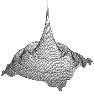

This tool is designed to create the artificial, nevertheless photometric realistic, frames. They are intended for modelling of various observation effects as well as for testing purposes.
munipack artificial [.. parameters ..]
Artificial frames are created by artificial photons having origin in physical principles and mathematical formulas rather than in nature. This approach can be very useful for understanding of true nature of many effects which can be else gathered by a plenty of observational experiences.
There is list of currently implemented features:
The frames are generated:
The properties of star images can be easy simulated for various quantum efficiency η of a detection apparatus (including detector itself), an exposure duration and a telescope diameter.
Both angular resolution and collecting area of a telescoped are proportional to diameter. The parameter --airy can set it directly, but better way is set diameter (via --diameter in meters) which sets both diffraction limit and input area.
An observed light intensity I(X) passing the clear (no clouds) Earth's atmosphere is attenuated proportionally of air-mass X according to the formula
I(X) = I0 e-k(X-1)
where I0 is an extra-atmospheric intensity. The extinction coefficient k depends on a spectral band.
The sky brightness (see below) is modelled by the same way (bZ is its zenit value)
b(X) = bZ e-k(X-1)
Turbulent motion in atmosphere creates large cells which slightly reflect light rays. The nature of turbulent motion is totally chaotic. There is a formula describing effect of chaotic moving of picture of a star due atmosphere during long exposures. It modelled star profile as function of air mass.
By Mr.Fries theory (very nice description has Electronic Imaging in Astronomy by Ian S. McLean), the seeing radius is modelled as
r'0 = r0 X0.6.
r'0 is an actual radius of stars at air-mass X, while r0 is the one at zenith.
These profiles known as point spread functions (PSF) are available:
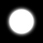
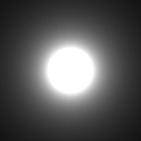
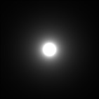
The plain diffraction pattern, representing response of an input aperture of a telescope without atmosphere seeing, can be generated as seeing spread with zero seeing parameter. It is difficult to expose it, even in laboratory, due to limited dynamical range of detectors.
The distribution of seeing is supposed as Gaussian and convoluted with actual diffraction profile. There are two methods convolution implemented:
All stars, on the image, are modelled with the same profile.
Non-circular star profiles are modelled by ellipse. Any ellipse is characterised by semi-major axis a (having radius meaning r0) and semi-minor axis b. b can not be specified directly: eccentricity 0 ≤ e < 1 is used instead; the parameter squeezes circle (e=0, a = b) to a line (e → 1).
Ellipsis is oriented to have its major semi-axis parallel to horizontal Cartesian axis by default. It can be optionally rotated by angle -90° < i ≤ 90°.
Non-circularity can be used to model imperfections in telescope tracking.
Background B(x,y) is modelled as a plane
b(x,y) = B0 + ΔBx (x - x0) + ΔBy (y - y0)
B(x,y) = N( b(x,y), Δb)
where B0 is a mean level (derived from --skymag) at centre of the picture x0, y0, N(b, Δb) is a function which makes a noise with Normal distribution. The parameters are mean level b and standard deviation Δb, which is computed as Δb = √ B0.
The optional gradient in background in counts per pixels is given by terms ΔBx, ΔBy (--sky-grad-x, --sky-grad-y). It can do modelling of a light pollution (by Moon). The common values for gradients are of order 0.0001 … 0.001 (negative values means negative slope of the plane in given direction).
| value [mag/arcsec2] | light conditions |
|---|---|
| above 22 | natural sky, high-altitude observatory |
| 22 | dark place, excellent night |
| 21 | countryside sky, average night |
| 20 | suburban sky, poor night |
| 18 | urban sky, full Moon |
| under 17 | city sky, twilight |
Values in the table are rought and determined by my observing experiences (wiki page).
Field stars are generated by a random number generator, if no -c option (a catalogue) is presented. Catalogue star coordinates and magnitudes are used otherwise.
Rectangular (without projection) coordinates of the stars has uniform distribution in ranges given by a frame size. The standard Fortran random number generator, with no initial seed, is used.
Magnitude distribution, meaning a probability to found number of stars in given magnitude interval per square degree, is modelled as an exponential function with a cut-off to prevent Olbersʼ paradox. I derived a rough approximation of the observed (surface) distribution of stars by brightens from DR1 by Gaia mission:
Σ(m) = 10-4 · e1.1m [□°], m < m0,
(the symbol □° designates square degree). The cut-off m0 is given by --maglim parameter. Large values of m0 and large field of view can effectively exhaust the computer memory.
The distribution approximation must be considered as an effective description. Stars are distributed over our sky very non homogeneously. Standard galaxy textbooks (like Binney's & Merrifield's Galactic Astronomy) gives more extensive description with references.
The artificial tool has three models of light curves included. The model of the pulsating star δ Cep (data computed by Mérand et al.) and the eclipsing binary star Algol (observed by Kim, Ho-Il). Both the curves has been approximated by Fourier series. The last model is a simple cosine wave.
There is also possibility to define own Fourier series approximation of light curves which is suitable for wave-like patterns. Do create a FITS table with format similar to fourier.lst. The table contains real Fourier coefficients an, bn. If the coefficients are estimated from measured data with noise, any appearance of high-order terms indicates inappropriateness of Fourier approximation. I can't recommend use on curves with sharp edges as Algol-like objects has. Note. The Fourier approximation gives very good approximation of Cepheids but is not very suitable for Algoids. The spline approximation can be recommended in that case.
Universal flux-time pattern is implemented as a time series table. It can represent a periodic object like Algol star or exoplanet transition, but it can also model an non periodic behaviour like a supernova explosion or an optical afterglow. The usage is described in Light Curves section of Overview.
This artificial tool implements models of elliptical galaxies. A radial profile have Sérsic profile (generalised de Vaucouleurs profile). A shape (nearly circular or nearly lenticular) is given by the Hubble classification; an orientation and shape of ellipticity is the same as for PSF of stars. All parameters are specified in the particular galaxy catalogue file. See Artificial sky for examples.
Every generated frame is marked by a symbol which indicates its artificial origin to prevent potential confusion. The mark can not be hide.
  $ munipack artificial
  $ xmunipack artificial.fits
Overview comes with more useful examples.
The table has similar format as the time-series table. It contains magnitudes (optionally, with errors) with columns: TIME,MAG,MAGERR. Records in the table must be sorted in time-increasing order. Overview describes its application.
This table contains two valid columns with Fourier series approximation of a light curve. The columns are: first is the real and second the imaginary part of Fourier complex coefficient. The text file fourier.lst demonstrates an instance of data (NAXIS2 must be updated when modified). A FITS file, required by --lc-fourier, will be created as
$ munipack fits --restore fourier.lst
Overview of Artificial sky, Artificial Sky … (seminary talk), Common options.